Working with Large Data Sets

This tutorial provides a walk-through of managing a large data set in R.  The sample data set used is on Precipitation in the Great Lakes Region retrieved from GLERL.  It is a multi-tab excel file that needs to be cleaned up in R before it can be used efficiently.  General methods of dealing with large datasets and the problems one can run into are included so that information in this tutorial can be applied to various types of data.

Glossary of terms used for this data set
Data file used: Precip_Basin

1. Loading the data file:
   There are several methods for reading in data files of various types (txt, csv, xlxs, etc.), but for this example we are working with an excel data set so will use the function read.xlsx().  This function will load a file from the current directory set in R, so before anything else we need to set the directory.  We also need to download an additional package in R and call it out from the library to use the read.xlsx() function.

   # Set directory
   setwd("~/1-R")
   
   # install and load packages to read xlxs files
    install.packages("xlsx")
    library(xlsx)

   Now R is set up to read in the excel file.  We will begin with just one tab in the file called ‘SUP_mm’ or the precipitation over Lake Superior in millimeters.  This is the second tab in the excel file.

   # Read xlsx file data
   P <- read.xlsx("Precip_Basin.xlsx", sheetName = 'SUP_mm')

   This function will read in the raw data as is.  This needs some cleaning up before we can work with it.  In the original file you’ll notice there are three lines of header in every tab that are unnecessary here, so we will skip straight to the fourth line by including the argument startRow = 4, then specifying that we still have column headers with the argument header = TRUE.  So now we have one line that will organize our data neatly when it is read in.
   

   # Read xlsx file data + headers
   P <- read.xlsx("Precip_Basin.xlsx", startRow = 4, header = TRUE, sep = ",", sheetName = 'SUP_mm')

2. Cleaning up the data set
   If you scroll to the edges of the data set you’ll see there are NA values where there were blank cells in the original excel file. To eliminate these we use the command na.omit and specify that we only need the first 14 columns.
   

   # Eliminate N/A values from data file
   P <- na.omit(P[1:14])

   Now there are still 3 rows at the bottom of the file that are separate from the rest of the data.  They are values for mean, max, and min precipitation values for every month.  This is still useful data so we can put it into another data variable, Pdata, while eliminating it from our main data variable, P.
   

   # Store mean max min data in separate data set
   P_data <- P[114:116,]
   
   # Eliminate mean max and min (aka: rows after 113) from data set
   P <- P[1:113,]
   

   The data set looks clean now, but if you open the drop down button beside the data you’ll see that all the months are classified as numerics while the year column is classified as a factor.  This will cause problems later with plotting and manipulating the data, so we will convert ‘Year’ first from a factor to a character and then to a numeric to match the rest of the data.  It needs to be converted to a character first to conserve the values that are there.  If it is converted straight to a numeric it will make the values into corresponding row numbers 1 through 113 instead of the actual year, and we do not want this.
   

   # Convert factors to numerics
   
   P[,1]<-as.character(P[,1])  # without this- years are converted to 1-114
   P[,1]<-as.numeric(P[,1])

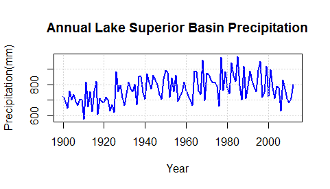
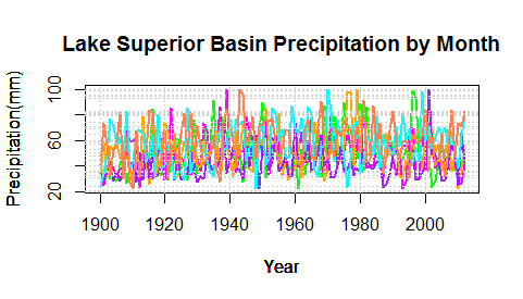
3. Using the data
   Now the data is clean and formatted to be easily usable.  This can be seen by plotting some of the data.  We can also make columns of data, like the year and the months easier to call by assigning them to variable names.

   # Assign variables
   year <- P[,'Year']
   jan <- P[,'JAN']
   feb <- P[,'FEB']
   mar <- P[,'MAR']
   apr <- P[,'APR']
   may <- P[,'MAY']
   jun <- P[,'JUN']
   ann <- P[,'Total']

   
   Plotting annual data:
   

   # plot Annual Precipitation
   plot(year,ann,
        type = "l",
        #ylim = c(0, 1050),
        main = 'Annual Lake Superior Basin Precipitation', 
        xlab = 'Year',
        ylab = 'Precipitation(mm)', 
        col = "blue", 
        lwd = 2)
   grid()
   par(new = F)

   
   Plotting multiple data strings at once:
   

   # Plot Precip values
   
   # jan
   plot(year,jan,
        type = "l",
        main = 'Lake Superior Basin Precipitation by Month', 
        xlab = 'Year',
        ylab = 'Precipitation(mm)', 
        col = "green", 
        lwd = 2)
   grid()
   par(new = T)
   
   # feb
   plot(year,feb,
        type = "l",
        axes = F,
        xlab = 'Year',
        ylab = 'Precipitation(mm)',
        col = "magenta", 
        lwd = 2)
   grid()
   par(new = T)
   
   # mar
   plot(year,mar,
        type = "l",
        axes = F,
        xlab = 'Year',
        ylab = 'Precipitation(mm)',
        col = "orange", 
        lwd = 2)
   grid()
   par(new = T)
   
   # apr
   plot(year,apr,
        type = "l",
        axes = F,
        xlab = 'Year',
        ylab = 'Precipitation(mm)',
        col = "purple", 
        lwd = 2)
   grid()
   par(new = T)
   
   # may
   plot(year,may,
        type = "l",
        axes = F,
        xlab = 'Year',
        ylab = 'Precipitation(mm)',
        col = "cyan", 
        lwd = 2)
   grid()
   par(new = T)
   
   # jun
   plot(year,jun,
        type = "l",
        axes = F,
        xlab = 'Year',
        ylab = 'Precipitation(mm)',
        col = "coral", 
        lwd = 2)
   grid()
   par(new = F)